QuestDB, an alternative for storing your financial time series.
Oct 29, 2025
Over the past two weeks, I’ve enjoyed some much-needed rest and time to reflect on my personal projects. One ongoing challenge has been efficiently storing financial time series data for future analysis. Selecting the right storage format is crucial—especially when seeking open-source database engines as alternatives to the widely used and robust KDB+. I’ve had the opportunity to work with KDB+ and its intuitive q programming language, which is both powerful and user-friendly. However, as your projects grow and require greater scalability, you’ll quickly realize that KDB+ comes with licensing costs. While these costs are justifiable for medium to large-scale initiatives, they may not be ideal for personal or smaller-scale projects where you want to start lean and scale gradually. Even KX acknowledges this in their own blog, offering a brief comparison between KDB+ and QuestDB—see their analysis here. For those looking to balance capability with cost, exploring open-source alternatives becomes essential.
In my projects, I routinely manage large volumes of time series data at various granularities—seconds, minutes, and days. While some may suggest aggregating these series in memory for time scaling, this approach introduces significant computational overhead. To address this, I maintain parallel copies of different frequencies, always seeking a robust database engine capable of handling such workloads efficiently. After extensive testing over several weekends, I discovered a solution that has consistently met my requirements: QuestDB.
QuestDB is an open-source time-series database designed for high-performance storage and retrieval of time series data. Its intuitive user interface eliminates the steep learning curve often associated with specialized time-series solutions. While there are other options available, my experience with QuestDB has been particularly positive. For context, I currently manage approximately 80 time series, each updated at second-level frequency from 08:30 to 18:00 daily, over a period of three months. Even when executing broad queries such as SELECT *, QuestDB has delivered reliable performance without issue. Importantly, it leverages standard SQL for data retrieval, making it accessible and straightforward for users familiar with relational databases.
⚠️ Warning :: I got inspired to share this information in case may be useful to somebody else. This post is not intended to benchmark QuestDB, but explaining how to install it, and even better, how to store your financial timeseries data in an external pen drive, it’s pretty easy, you shall see. A plus added is a small backtesting conducted using the data ingested in QuestDB.
Installation
The instalation is nothing different to what’s explained in their webpage, so I’m not going to dive deep on that, that by the way is pretty nice explained and explicit for each operative system. In my case it is Linux. Instead, I want to emphasizessssssss on how it works once you want to create a basic database for storing, i.e. crypto currency price timeseries. Once downloaded, you can run the following commands.
- Unzip the tar.gz file, that will create a new folder. Please notice the version of this example is QuestDB 9.1.0, therefore, if more recent version is released, you need to change the version once unzipped. The unzipped folder is namedd
questdb-9.1.0-rt-linux-x86-64in this example.> tar -xvzf questdb.tar.gz - Moving the unzipped folder to the folder of your preference. In my case, it is
opt/questdb, taking into consideration the linux directory functionality, as explained here.> mv questdb-9.1.0-rt-linux-x86-64 opt/questdb - Once the folder is moved to
opt/questdb, you will notice there is a file namedbin/questdb.shwithin. This shell file is in charge of starting or stopping the database engine daemon. So my suggestion is to avoid referring always to the absolute path, just adding an alias in your.bashrcfile (more info here). For instance as follows.
alias questdb_engine='/opt/questdb/questdb-9.1.0-rt-linux-x86-64/bin/questdb.sh'
QuestDB database creation
Now, the goal is to store the data in a pen drive, such that is also available in any other machine with QuestDB installed. The reader may be thinking “why do not even allow QuestDB being portable”?. I though about this option, but in this use case the data is the king, and QuestDB the King’s sword. So, let’s create it assuming you have a pen drive that is accessible in the path /media/<username>/<pendrive-name>, once mounted in linux. Internally, you have created a new folder named my-timeseries/, therefore, the complete path is /media/<username>/<pendrive-name>/my-timeseries/. Let’s create the database in there.
The alias questdb_engine was created above. Thereby, you will be able to run the engine storing metadata and data in the pendrive by runnning the following command.
> questdb_engine start -d /media/<username>/<pendrive-name>/my-timeseries/
Or, if you prefer to run without an alias, you may execute it directly with the command below.
> /opt/questdb/questdb-9.1.0-rt-linux-x86-64/bin/questdb.sh start -d /media/<username>/<pendrive-name>/my-timeseries/
Voila!, if you see an output as shown below, you have created your database in an external drive!!. I told you it is pretty easy!
JAVA: /opt/questdb/questdb-9.1.0-rt-linux-x86-64/bin/java

     ___                  _   ____  ____
    / _ \ _   _  ___  ___| |_|  _ \| __ )
   | | | | | | |/ _ \/ __| __| | | |  _ \
   | |_| | |_| |  __/\__ \ |_| |_| | |_) |
    \__\_\\__,_|\___||___/\__|____/|____/
                        www.questdb.io

    Web Console URL                 ILP Client Connection String

    http://172.17.0.1:9000          http::addr=172.17.0.1:9000;
    http://192.168.1.14:9000        http::addr=192.168.1.14:9000;
    http://127.0.0.1:9000           http::addr=127.0.0.1:9000;

QuestDB configuration files are in /media/<username>/<pendrive-name>/my-timeseries/conf
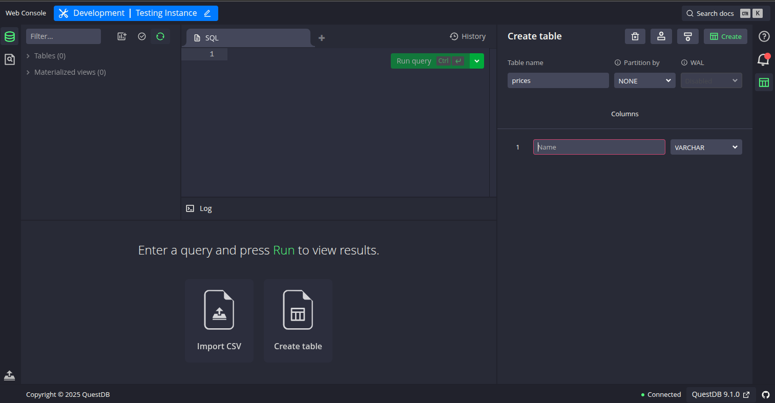
As you can see in the prompt above, an user interface via webbrowser to interact with your data is available via http://172.17.0.1:9000 url. You can click in the terminal or typing it in your web browser. It redirects to the nice user interface shown below, which is also quite intuitive if you already have experienced with SQL IDEs, but if you want more info take a look in this video in Youtube, and subscribe to the channel.
Experiment
Now, the UI looks nice, but what to do with all that in your pocket?. Let’s assume that you have the following timeseries in a csv file, and you would like to store it in your just created QuestDB database.
| date | close | volume |
|---|---|---|
| 20250313 15:30:00 Europe/Warsaw | 121.73 | 123702.34 |
| 20250313 15:30:01 Europe/Warsaw | 122.15 | 124100.12 |
| 20250313 15:30:02 Europe/Warsaw | 121.98 | 123950.87 |
| 20250313 15:30:03 Europe/Warsaw | 122.30 | 124210.45 |
| 20250313 15:30:04 Europe/Warsaw | 121.65 | 123800.56 |
| 20250313 15:30:05 Europe/Warsaw | 122.05 | 124050.23 |
| 20250313 15:30:06 Europe/Warsaw | 121.90 | 123900.77 |
| 20250313 15:30:07 Europe/Warsaw | 122.20 | 124180.34 |
| 20250313 15:30:08 Europe/Warsaw | 121.80 | 123850.12 |
| 20250313 15:30:09 Europe/Warsaw | 122.10 | 124120.65 |
Creation of your first table
As in many databases, you store data in tabular format by means tables. Those tables are created ad-hoc, as you wish or require. In this case, for abovementioned data, we can create the table executing the following command in QuestDB user interface (Center segment for sql queries), via form available in the right lateral panel, or even uploading a csv file directly in the web browser (button panel).
CREATE TABLE 'prices' (
  date TIMESTAMP,
  close FLOAT,
  volume FLOAT,
) timestamp (date) PARTITION BY DAY BYPASS WAL
DEDUP UPSERT KEYS(date);
This table will store the table mentioned as example. Some considerations are:
timestamp (date): Specifies that the date column is the designated timestamp for this table. QuestDB uses this to efficiently index and query time-series data. More information here.PARTITION BY DAY: Tells QuestDB to store data in daily partitions. This improves query performance and makes it easier to manage large time-series datasets. More details here.BYPASS WAL: Disables the Write-Ahead Log (WAL) for this table. WAL is used for durability and crash recovery. Bypassing it can improve write performance but may risk data loss if the server crashes before data is flushed to disk. Personally I do prefer having it enabled for low amounts of data dump. More details hereDEDUP UPSERT KEYS(date, file_path);: Enables deduplication, which ensures that if multiple rows have the same values for the specified key columns (here,date), only the latest row is kept in the table while updating the remaining ones. This helps prevent duplicate records, maintains data integrity, and simplifies updates when ingesting time series data from multiple or repeated sources. For more details, see the QuestDB deduplication documentation.
Then the forthcoming step is to use this table to store the data we receive from any source, for instance your broker via websockets.
Data Ingestion
The reader, you, may use the client provided by QuestDB in many different programming languages like Python, C++, Rust, Java, and others. However, during my own experiments I realized that for avoiding to use a streaming data pipelines like Kafka, RabbitMQ, Redpanda or any other, I’m allowed to use the ILP protocol. Beforementioned protocol refers to InfluxDB protocol, that facilitates the massive ingestion of data. Conversely to the client which conveyes data via HTTP protocol, limiting the number of records given the limit size of the payload, ILP protocol conveys the data in another way. The InfluxDB protocol conveys the information by organizing the data in plain text rows with some rules. Here is the same data in QuestDB ILP (Influx Line Protocol) format, ready for ingestion:
prices,close=121.73,volume=123702.34 1748413800000000
prices,close=122.15,volume=124100.12 1748413801000000
prices,close=121.98,volume=123950.87 1748413802000000
prices,close=122.30,volume=124210.45 1748413803000000
prices,close=121.65,volume=123800.56 1748413804000000
prices,close=122.05,volume=124050.23 1748413805000000
prices,close=121.90,volume=123900.77 1748413806000000
prices,close=122.20,volume=124180.34 1748413807000000
prices,close=121.80,volume=123850.12 1748413808000000
prices,close=122.10,volume=124120.65 1748413809000000
For more details of QuestDB ingestion visit them here.
Testing using Telnet
You can quickly test data ingestion into QuestDB using telnet and the ILP format. For example, to send the sample rows above to your prices table, open a terminal and run:
telnet localhost 9009
Once connected, paste the following lines (each as a single line, then press Enter):
prices,close=121.73,volume=123702.34 1748413800000000
prices,close=122.15,volume=124100.12 1748413801000000
After sending the data, close the connection with Ctrl+] then type quit. The rows will be ingested into QuestDB and available for querying.
Useful functions in C++ for ILP ingest
As you see is quite simple creating the information that is conveyed to QuestDB. Further more, it’s practically a transformation of a csv file. the first field corresponds to the name of the table where it is registered, namely prices, just created above. Subsequently, fields close and volume is referenced. Eventually, the last set of information corresponds to the date, that was stablished to be the partition of the table, but also expressed in microseconds, always. This is one remark that worths to mention, every column set as timestamp datatype, requires to be send in ILP protocol in microseconds. Thereby, an example of function that cast the datetime string in C++ is shown below.
#include <chrono>
#include <iostream>

long long to_nanoseconds_since_epoch(const std::string& datetime, const std::string& format = "%Y-%m-%dT%H:%M:%S") {
    std::istringstream ss(datetime);
    std::tm tm = {};
    ss >> std::get_time(&tm, format.c_str());
    if (ss.fail()) {
        throw std::runtime_error("Failed to parse datetime: " + datetime);
    }
    auto tp = std::chrono::system_clock::from_time_t(std::mktime(&tm));
    return std::chrono::duration_cast<std::chrono::nanoseconds>(tp.time_since_epoch()).count();
}
Furthermore, a function example that sends the string with all the rows constructed, is detailed below.
#include <sys/socket.h>
#include <netinet/in.h>
#include <arpa/inet.h>
#include <unistd.h>
#include <cpr/cpr.h>
/**
 * @brief Sends ILP data to a specified host and port over a TCP connection.
 *
 * This function is useful for writing the content of CSV files by transmitting
 * the provided ILP data string to a remote server using a TCP socket.
 *
 * @param host The IP address or hostname of the destination server.
 * @param port The port number to connect to on the destination server.
 * @param ilp_data The ILP data string to be sent, typically representing the content of a CSV file.
 */
void send_ilp(const std::string& host, int port, const std::string& ilp_data) {

    int sock = socket(AF_INET, SOCK_STREAM, 0);
    sockaddr_in serv_addr{};
    serv_addr.sin_family = AF_INET;
    serv_addr.sin_port = htons(port);
    inet_pton(AF_INET, host.c_str(), &serv_addr.sin_addr);

    if (connect(sock, (sockaddr*)&serv_addr, sizeof(serv_addr)) < 0) {
        std::cerr << "Connection failed\n";
        return;
    }
    send(sock, ilp_data.c_str(), ilp_data.size(), 0);
    close(sock);
}
With this set of functions you are ready to convey information to QuestDB, and then use it in any research that requires that information.
Using the information in Market Research
As any quant, this is just a small piece of the infraestructure required to have available information for any research. But let’s now assuming you want to use this information in a backtesting example, testing Bollinger Bands. Because it’s prototyping it’s pretty much easy to switch to python. Thus, the code is now as follows.
Libraries required
For this small test you require to install the following list of libraries
Perhaps you saw something interesting. We’re not necessarily using QuestDB client. This is because besides QuestDB client, it is also possible get access to the database via psycopg2 library, used for connection to PostgreSQL databases.
Basic Setup
The following lines refer to basic setup for this experiment. Quite standard, I’d say.
import psycopg2
import polars as pl
import numpy as np
import plotly.graph_objects as go
import matplotlib.pyplot as plt
import pandas as pd

pl.Config.set_tbl_formatting("ASCII_MARKDOWN")
pl.Config.tbl_float_precision = 6  # Show 6 decimals

TABLE = 'prices'
Database Connection
In this example, the connection to QuestDB is established using the psycopg2 library, which communicates with the database on localhost via the default port 8812. Unless you have configured custom credentials, the default username and password are used. If you are familiar with other database connectors in different programming languages, you will recognize the need to create a cursor to execute queries and manage communication between the client and the database engine.
conn = psycopg2.connect(
    dbname="qdb",
    user="admin",
    password="quest",
    host="localhost",
    port=8812
)
cur = conn.cursor()
Retrieving data
Now, the cursor is used to send an SQL sentence selecting the data for dates 2025-03-13 and 2025-03-14. But depending the data you have fed, you can change it to whatever period you have. Without getting into details, the condition to filter dates can be changed of course, to select a range of dates, you know what I mean. QuestDB natively can be connected via polars dataframe, as shown below.
sql_select = "SELECT to_str(date,'yyyy-MM-ddTHH:mm:ss') as date,  close, volume\n" \
                f"FROM {TABLE} \n" \
                "and to_str(date,'yyyy-MM-dd') in ('2025-03-13','2025-03-14')\n"

df_prices = pl.read_database(sql_select,connection=conn,)

df_prices = df_prices.with_columns([
    pl.col("date").str.strptime(pl.Datetime, "%Y-%m-%dT%H:%M:%S"),
    pl.col("extraction_date").str.strptime(pl.Datetime, "%Y-%m-%dT%H:%M:%S")
])
Calculating Bollinger Bands
To avoid reinventing the wheel, this example leverages the TA-Lib package for calculating technical indicators such as Bollinger Bands. The following code demonstrates how to perform this calculation. For a deeper understanding of the methodology and additional tips on testing combined strategies, refer to Technical Analysis for the Trading Professional by Constance Brown (Ch. 11).
A more formal notation is for bands can be found in the book titled Technical Analysis from A to Z, by Steven Achelis, in page 74, where these are described like:
\[UpperBand = MiddleBand + \left[n\cdot \sqrt{\frac{\sum_{j=1}^n(Close_j-MiddleBand)^2}{n}} \right]\] \[LowerBand = MiddleBand - \left[n\cdot \sqrt{\frac{\sum_{j=1}^n(Close_j-MiddleBand)^2}{n}} \right]\]Where $MiddleBand$ is the moving average $MA$ in our experiment. This logic can be easily coded and tested using TA-Lib, allowing for rapid prototyping and performance evaluation of the strategy. It also provides different moving average methods, that adds flexibility to the experiment.
upper, middle, lower = talib.BBANDS(df_prices['close'], matype=MA_Type.SMA, timeperiod=14)
pl.Config.tbl_float_precision = 6  # Show 6 decimals
df_prices = df_prices.with_columns(
    pl.Series("upper", upper),
    pl.Series("middle",middle),
    pl.Series("lower", lower)
)
To recap, Bollinger Bands consist of a moving average (MA) as the central baseline, with the upper and lower bands defined by the formula $\text{MA} \pm \gamma \cdot \delta$, where $\text{MA}$ stands for Moving Average, $\delta$ represents the standard deviation and $\gamma$ is the number of standard deviations selected for the strategy. In this example, a moving average period of 14 data points is used.
Plotting the results
fig = go.Figure()

fig.add_trace(go.Scatter(
    x=df_prices['date'].to_numpy(),
    y=df_prices['close'].to_numpy(),
    mode='lines',
    name='Close'
))
fig.add_trace(go.Scatter(
    x=df_prices['date'].to_numpy(),
    y=upper.to_numpy(),
    mode='lines',
    name='Upper Band',
    line=dict(dash='dash')
))
fig.add_trace(go.Scatter(
    x=df_prices['date'].to_numpy(),
    y=lower.to_numpy(),
    mode='lines',
    name='Lower Band',
    line=dict(dash='dash')
))

fig.update_layout(
    title=f'{TABLE} : BollingerBands ',
    xaxis_title='Time',
    yaxis_title='Price',
    xaxis=dict(
        tickformat='%m/%d-%H:%M:%S'
    ),
    width=1600,
    height=900
)

fig.show()
Backtesting the strategy
The core strategy involves entering a long position when the price crosses below the lower Bollinger Band, and entering a short position when the price crosses above the upper Bollinger Band. This approach aims to capitalize on potential price reversals at the extremes of volatility. For implementation, the VectorBT library is utilized due to its intuitive interface and flexibility for backtesting various scenarios.
The entry and exit signals are defined as follows:
- Long Entry: When
price < lower_bandor $P < \text{MA} - \gamma \cdot \delta$ - Short Entry: When
price > upper_bandor $P > \text{MA} + \gamma \cdot \delta$
l_entries = df_prices['close'] < df_prices['lower']
l_exit = df_prices['close'] > df_prices['upper']
A small slipage is added as proportion of the last observed price, but before we need to create the noise.
# Slipage
np.random.seed(42)
prices_size = df_prices.shape[0]
slippage = pd.Series(np.random.uniform(0, 0.0015, prices_size), index=df_prices['date'])
Then the portfolio backtesting is created adding entry and exit fees also, as proportion of the total order amount (%). Both cases set as 0.1% of the order amount, as follows. Furthermore, it is set a maximum proportion of available cash that can be used for trading if a signal suggests it, set as 30%. The list of trades can be accessed via portfolio.trades.records.
portfolio = vbt.Portfolio.from_signals(
    df_prices['close'],
    l_entries,
    l_exit,
    slippage=slippage,  # stochastic slippage per bar (% of price at that moment)
    fees=0.001, # Percentage of trade
    size=0.3 # Using the % in this parameter, over available cash
)

trades = portfolio.trades.records
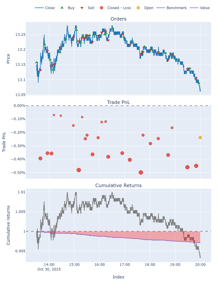
Eventually, you can see the portfolio performance and plots showing the historical performance in the backtesting.
- Show the plots
portfolio.plot().show() - Display performance metrics
stats = portfolio.stats()
print(stats)
Below an example for another date. The result of this example is not promising, but that’s the exciting part, conducting the appropriate fine tuning which I’ll talk about in forthcoming posts.
Start                         2025-10-30 13:30:00
End                           2025-10-30 19:59:50
Period                            0 days 06:30:00
Start Value                                 100.0
End Value                               99.708598
Total Return [%]                        -0.291402
Benchmark Return [%]                    -0.608365
Max Gross Exposure [%]                    3.98698
Total Fees Paid                          0.202055
Max Drawdown [%]                         0.291248
Max Drawdown Duration             0 days 06:27:50
Total Trades                                   26
Total Closed Trades                            25
Total Open Trades                               1
Open Trade PnL                          -0.009346
Win Rate [%]                                  0.0
Best Trade [%]                          -0.069792
Worst Trade [%]                         -0.499154
Avg Winning Trade [%]                         NaN
Avg Losing Trade [%]                    -0.284596
Avg Winning Trade Duration                    NaT
Avg Losing Trade Duration         0 days 00:09:02
Profit Factor                                 0.0
Expectancy                              -0.011282
Sharpe Ratio                          -122.161294
Calmar Ratio                           -336.62527
Omega Ratio                               0.74954
Sortino Ratio                         -155.247853
dtype: object
Closing the cursor and the connection
It is a good practice to finish the connection once it is not used anymore, specially to release resources. It can be done as follows.
cur.close()
conn.close()
Stopping QuestDB
As you remember you have created an alias named questdb_engine. You can use the same to stop the daemon once you don’t need it anymore, thereby you close any connection. Just remember start the daemon again if you want to use it again.
> questdb_engine stops
Key Takeaways
- QuestDB offers a compelling, cost-effective alternative to the KDB engine for time-series data storage and straightforward analysis.
- Deduplication of records allows to reduce the amount of execution code in logic layer managing duplication of records, particularlly useful in time series when price may be corrected in different batches but pointing out same timestamp and ticker.
- External storage support: QuestDB may store both data and metadata on external devices by specifying a simple parameter at daemon execution, enhancing portability and flexibility.
- SQL compatibility: The familiar SQL language makes it easy to get started and interact with the database, especially for those new to QuestDB.
- Optimized for time-series workloads: While QuestDB is designed for efficient time-series data handling, it does not provide the same breadth of built-in time-series functions as KDB.
- PostgreSQL connector support: QuestDB can be accessed using standard PostgreSQL connectors, simplifying integration and management across various programming environments.
- Efficient data ingestion: The Influx Line Protocol (ILP) enables high-performance ingestion of large volumes of time-series data, outperforming traditional HTTP-based methods for bulk operations.
Hope this information is useful for you. Any doubt not hesitate reaching me out via LinkedIn, I’ll be really happy to help.